Difference between revisions of "Conditional formatting - User defined benchmark column"
| Line 2: | Line 2: | ||
| − | First, select the desired base column, then select '''Set Base Column''' under '''Base Column''' from the ''' | + | First, select the desired base column, then select '''Set Base Column''' under '''Base Column''' from the '''Spreadsheet''' ribbon. |
[[File:Conditional-formatting user-defined-benchmark-column set-base-column.jpg|thumb|center|x350px]] | [[File:Conditional-formatting user-defined-benchmark-column set-base-column.jpg|thumb|center|x350px]] | ||
| + | [[File:Cond-format user-defined-benchmark set-base-column.jpg|thumb|center|x350px]] | ||
After the base column is set, select either a certain row/column/section or the entire spreadsheet to compare to the base column. The entire spreadsheet can be selected by clicking on the corner between A and 1. Next, select the '''Apply Conditional Formatting''' option from the '''Appearance''' ribbon. | After the base column is set, select either a certain row/column/section or the entire spreadsheet to compare to the base column. The entire spreadsheet can be selected by clicking on the corner between A and 1. Next, select the '''Apply Conditional Formatting''' option from the '''Appearance''' ribbon. | ||
Revision as of 13:45, 31 July 2013
Conditional Formatting has been a well used tool since its introduction to mTAB and the ability to benchmark responses against the total has proven popular too. Always looking to provide the greatest flexibility, mTAB has now been enhanced in this area, now allowing the user to not only benchmark against the total (as explained in a previous article, Conditional Formatting Overview), but against any other column or row within the spreadsheet.
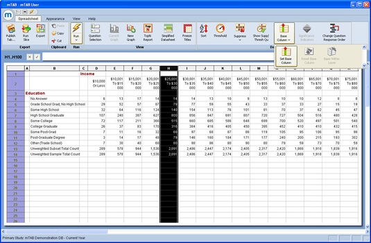
First, select the desired base column, then select Set Base Column under Base Column from the Spreadsheet ribbon.
After the base column is set, select either a certain row/column/section or the entire spreadsheet to compare to the base column. The entire spreadsheet can be selected by clicking on the corner between A and 1. Next, select the Apply Conditional Formatting option from the Appearance ribbon.
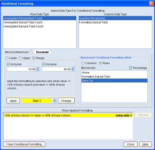
In the dialog that pops up, select the Threshold tab, and set your threshold values, upper, lower, or range. The Benchmark Conditional Formatting within section is where you now have the option of selecting a base column, Base Col, for the comparison, either as a value or percentage. Once you click Apply the selection appears in the list of conditional formats. Then click Close.
Once the base column and thresholds are set, the results are displayed based on your criteria.

