How to use Slice
Slice is an extension module to the mTAB software that enables the export of data at respondent level. It gives users the ability to examine and filter the data in mTAB, but then focus on a particular area of interest and export only the relevant questions and respondents from mTAB in either SPSS, SAS or ASCII file format for further analysis. The analyst is then free to apply the advanced statistical methodologies found in these software packages to that part of the research data under scrutiny.
You will find the ‘Slice’ command under mTAB’s File menu. Before selecting this option, you may need to do some preparation work to ensure that you only slice the specific data required for your further analysis.
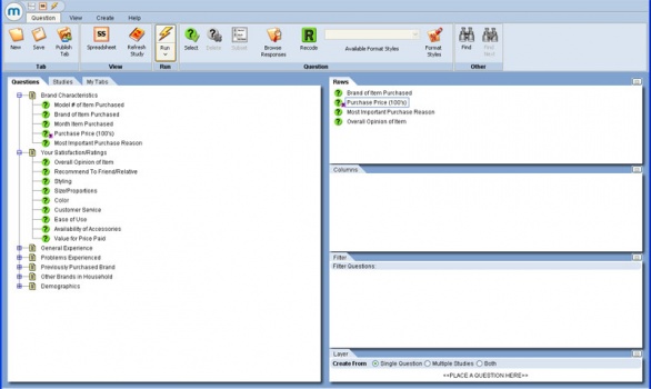
If you wish to slice only a selection of the questions available in the database, we suggest that the questions required be placed on the Rows tab in mTAB.
Questions can also be added to the Columns and Layer panels but it is easier to see which variables will be sliced by keeping them all in one place, such as the Rows tab as suggested. If no questions are placed on the Rows, Columns or Layer, Slice will output all questions contained within the database.
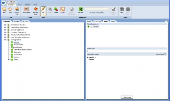
If you wish to define the respondents to be sliced out of the database, place relevant questions on the Filter tab in mTAB and subset accordingly.
If no Filter questions are added, Slice will by default output all respondents contained within the database.
Once your preparation work for the slice is complete in the mTAB question selection view, go to the File menu and select Run Slice.
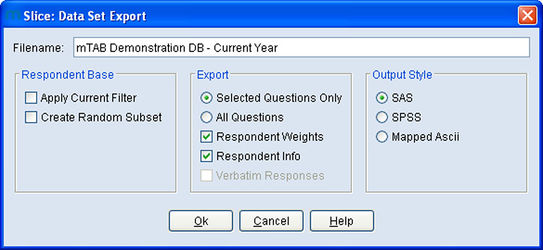
The Slice: Data Set Export dialog will appear.
Your first task is to provide a file name for your Slice job.
By default, Slice will apply the name of the database from which the data is being sliced.
This can be changed by simply editing the title shown in the File name box.
You now need to finalize the Slice Job by selecting the appropriate Respondent Base, Export and Output Style.
Respondent Base:
If both the ‘Apply Current Filter’ and ‘Create Random Subset’, options are left unchecked, Slice will output all respondents included in the database.
Select the ‘Apply Current Filter’ option if you wish to export only the respondents that pass the filter criteria that has been set up as part of the preparation work. If no questions have been added to the Filter, this option will not be available.
Select the ‘Create Random Subset’ option if you wish to limit the number of respondents to a set number. On selecting this option Slice will show the Total sample count that could be sliced and ask you to input the number of respondents that you require to be randomly generated.
Export:
Choosing ‘Selected Questions Only’ slices only the questions selected on the rows, columns or Layer as part of the Slice preparation. If no questions have been selected in mTAB, this option will not be available.
Choosing ‘All Questions’ slices all of the questions in the database.
Choosing ‘Respondent Weights’ will ensure the weighting coefficients for each respondent is included in the slice job. If there is no weighting scheme applied to the database, this option will not be available.
Choosing ‘Respondent Info’ asks Slice to include non-analytical data not shown as questions in the database, such as the respondent identification number, to be included in the Slice Job.
Choosing ‘Verbatim Responses’ allows the verbatim answers to be included in the slice job, instead of the post-coded responses. If the verbatim responses have not been incorporated into the database, this option will not be available.
Output Style:
The ‘SAS’ option creates a .DAT and a .SAS file which can be imported directly to SAS.
The ‘SPSS’ option creates a .DAT and a .SPS file that can be imported into SPSS to create a .SAV file.
If exporting in SPSS format, please also refer to Importing a SLICE file into SPSS.
The 'Mapped ASCII' option creates a .DAT fixed field, fixed record ASCII format file and a .MAP description file.
Processing the Slice Job
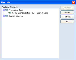
After selecting the options above, select OK and the Slice job will be sent for processing. This may take a few minutes but you can determine the status of each Slice job by selecting Slice Jobs from the File menu.
Each Slice job will be shown as either Processing or Completed in the dialog box as shown.
Once your slice job has moved to Completed Jobs you can download the created files to your PC. Highlight the completed Job and select Download. You will then be asked to choose a folder to which the files will be saved.
NOTE: By using the Slice module you could potentially be creating very large data files, particularly if you choose to slice an entire mTAB database. Also, please be aware that mTAB databases can contain complicated variables, such as Group Questions, which may not easily export to SPSS, SAS or other database systems, as they do not support these unique data structures.
Interpreting the output of Slice
Downloading the slice job to your PC, will result in the creation of three files. For example, if we selected the Mapped Ascii output options, files would be created in our local directory (as selected when we downloaded) and the three files would be called:
- MC97Q1.DAT - The “raw” ASCII file in fixed field, fixed record length format.
- MC97Q1.MAP - A file documenting the MC97Q1.DAT file.
- MC97Q1.SMP - A “Saved Sample” file. This file is used if you need to create a second slice of data and identify the exact same respondents as a prior slice. Unless you need to create two or more “slices” representative of the same respondents, you can ignore this file.
The DAT and MAP files should be viewed with an ASCII file editor.
Interpreting the MAP file
An example MAP file is shown below:
Data File="mc97q1.DAT" "Record Length =", 50
"Field", "Start", "Width", "QMnem", "TMnem", "Group ID", "Group Ct", "MultiCount", "Weight" "Respondent ID", 1, 5 "Regular Weight", 6, 12, "WTS_REG", "WEIGHT" "Repurchase Loyalty Weight", 18, 12, "WTS_REPUR", "WEIGHT" "Sales/Owner Loyalty Weight", 30, 12, "WTS_SOS", "WEIGHT" "Purchased Vehicle (Mailout Label)", 42, 5, "VC_MLCODE", "MOLC97Q1", -1, 1, 1, "WTS_REG" "Sex", 47, 1, "DMO_SEX", "MALEFEMA", -1, 1, 1, "WTS_REG"
"MOLC97Q1" "Chrysler Cirrus", 472 "Chrysler Concorde", 397 "Chrysler LHS", 436 "Chrysler Sebring Coupe", 10323 "Chrysler Sebring Conv", 10372
... and so on ...
"MALEFEMA" "No Answer", 0 "Male", 1 "Female", 2
As mentioned previously, the MAP file documents the contents of the DAT file. The rows in the MAP file shown below:
"Respondent ID", 1, 5 "Regular Weight", 6, 12, "WTS_REG", "WEIGHT" "Repurchase Loyalty Weight", 18, 12, "WTS_REPUR", "WEIGHT" "Sales/Owner Loyalty Weight", 30, 12, "WTS_SOS", "WEIGHT" "Purchased Vehicle (Mailout Label)", 42, 5, "VC_MLCODE", "MOLC97Q1", -1, 1, 1, "WTS_REG" "Sex", 47, 1, "DMO_SEX", "MALEFEMA", -1, 1, 1, "WTS_REG"
... represent each of the fields in the DAT file. In this example, there were six fields output including respondent id, regular weight, repurchase loyalty weight, sales/owner loyalty weight, Purchase Vehicle (mailout label), and Sex. mTAB will always slice out the respondent id and any weight fields in addition to any selected questions. In this example, the selected questions were Purchase Vehicle (mailout label) and Sex.
The two numbers after each of these questions represents the column position and field width of this data as found in the DAT file. For example, the codes for Purchase Vehicle (Mailout Label) are found at the 42 column of the DAT file in a 5 character wide field.
The code tables associated with these positions are documented beneath the layout information. For example, the code table associated with Purchased Vehicle (Mailout Label) is called MOLC97Q1. The code-to-vehicle description is shown in the MOLC97Q1 table beneath the layout as shown below:
"MOLC97Q1" "Chrysler Cirrus", 472 "Chrysler Concorde", 397 "Chrysler LHS", 436 "Chrysler Sebring Coupe", 10323 "Chrysler Sebring Conv", 10372
Therefore, if a code of 397 was found at the position 47, field width of 5 in the DAT file, we can conclude that the respondent purchased (Purchased Vehicle question) a Chrysler Concorde.
There are additional instructions required to interpret the ‘slice’ output for Group questions. Group questions, which are typically denoted with a (Gn) (e.g. Rated Vehicle (G1) ) within the question text, contain an array of responses for per each respondent. Group questions are sometimes referred to as ‘grid’ questions, corresponding to how the data is collected from a paper survey. For example:
| Please rate 1-5 | Brand A | Brand B | Brand C |
| Exterior Rating | 5 | 5 | 4 |
| Interior Rating | 4 | 1 | 3 |
| Ride Rating | 4 | 3 | 2 |
| Quietness Rating | 5 | 3 | 5 |
| Value Rating | 3 | 3 | 5 |
... would be represented in mTAB as five separate questions, all designated with the (Gn) marking; Rated Brand (G1), Exterior Rating (G1), Interior Rating (G1), Ride Rating (G1), Quietness Rating (G1), and Value Rating (G1). Expect in rare occasions, you will always include the main (in this example , Rated Brand) question along with at least one other group question in your tabs.
Slicing group questions returns individual fields for each of the group responses. Therefore, continuing with our example, the question Rated Brand (G1) would slice into the following fields:
Rated Brand (G1) (1) Rated Brand (G1) (2) Rated Brand (G1) (3)
... with each field containing the response for that brand. The response found in the field, in this case a brand code, would be interpreted by looking at the associated table for that question.
It is important to realize that the association between the group responses carry across the group questions. All group questions variables labeled as (2), for example, refer to the same group response. By way of example, let’s suppose the data in field Rated Brand (G1) (2) was a code of 32 and the data in field Exterior Rating (G1) (2) was a 5. It is important to understand that the (2), referring to the second group response, means that the respondent gave an exterior rating of ‘5’ for brand code 32. The respondent’s rating found in field Exterior Rating (G1) (3) is associated with the brand code found in Rated Brand (G1) (3) and so on.


